Bruker TruLive3D

Training manual for the Bruker TruLive3D Light Sheet Microscope. Acknowledging the Arnold & Mabel Beckman Foundation for their support in acquiring the Bruker TruLive3D microscope.

• Bruker TruLive3D training protocol
• Bruker TruLive3D specifications and primary uses
• 1. Bruker TruLive3D start-up procedure
• 2. Bruker TruLive3D microscope overview
• 3. Bruker TruLive3D Lux-Bundle overview
• 4. Bruker Trulive3D calibration
• 5. Bruker TruLive3D Finding the sample
• 6. Bruker TruLive3D Experiment
• 7. Bruker TruLive3D Data management
• 8. Bruker TruLive3D Using the photo-manipulation (PM) feature
• 9. Bruker TruLive3D shut-down procedure
• Bruker TruLive3D Sample preparation guidelines
• Bruker TruLive3D emission filters and fluorophores spectrum
• Bruker TruLive3D Data management pipeline
• Bruker TruLive3D Data visualization in Fiji

Bruker TruLive3D training protocol

Training Program 

Bruker TruLive3D Light Sheet Microscope 

 

Session 1 – Instrument and Operation Overview*

Microscope Startup Procedure 

Microscope overview 

Optical Path Overview 

Bruker Lux-Bundle Overview  

Microscope calibration 

* This session is now optional! The calibration will be performed by Beckman center Staff if you prefer not to learn how to do it. You can always book a training to learn how to do it later and be more autonomous on the instrument.

Session 2 – Setting up an experiment 

Review of microscope calibration 

Sample finding 

Setting up an experiment in LuxBundle 

Data saving options 

 Data analysis in LuxBundle 

     1. Image viewing in LuxBundle

     2. Image processing in LuxBundle: learn how to create separate imaris headers for each stack

 Shutdown Procedure and Calendar Access 

     1. System shutdown 

     2. Cleaning procedure 

     3. Calendar access 

 

Session 3 – User-led Session 

     2. Notify the Instructor as to the date/time of the session 

     3. Reserve at least two hours 

     4. Turn on the microscope 

     5. Load your sample 

     6. Calibrate the instrument 

     7. Find your sample 

     8. Set up an experiment 

The instructor will check in on you throughout to offer assistance 

Optional Session – Photomanipulation module 

 

     2. Beam Calibration 

     3. Photo-Manipulation Module 

     4. Calibration of the PM module 

     5. Load in your sample 

     6. Find your sample on the SpinView software with the BlackFly camera 

     7. Explore the different photomanipulation options 

     8. Set up an experiment with a photomanipulation event 

Bruker TruLive3D specifications and primary uses

Bruker TruLive3D main specifications

• The TruLive3D has 4 imaging channels at 405nm, 488nm, 561nm, 640nm. 

• The imaging objective is 25X 1.1NA water immersion. The magnification changer does not change the NA of the system. 

• The system is corrected for chromatic aberrations for the visible wavelengths but does present a shift for the UV 405. This can be corrected with processing. 

• The sample dishes are index matched to water so as long as the medium we use is index matched to water we can image with full resolution.

Bruker TruLive3D primary uses

• The instrument is primarily designed to image organoids or spheroids up to less than a millimeter in size.
• The instrument can be used for live cells, live small embryos, zebra fishes
• The instrument is NOT designed to image cleared tissues for the following reasons:
  • The clearing process uses chemicals that can attack the glue of the imaging objective
  • The clearing process matches the index of refraction of the tissue to that of the clearing medium. This results in indexes of refraction way beyond the index of refraction of water.
  • To have a tissue matched to the index of refraction of water, one could use expansion microscopy in some cases but the end results would likely be too large to image at once in the sample dishes.

1. Bruker TruLive3D start-up procedure

 

a.      Turn on the microscope

In case of emergency, push the big red button: it turns off the entire system. When you turn it back on, turn it counter clockwise until it is pulled all the way.

b.      Turn on the two cameras

c.      Fill the sample chamber with DI water using the squeezy bottle. You should submerge the illumination objective. If you happen to pour too much water, use the syringe to drain the excess out. Always use the syringe to drain water only, do not re-inject water inside the chamber. Use the bottle of DI water to add water. If you accidentally really poured too much water and need to empty the syringe in the DI waste becher, make sure you hold the pipe above the sample chamber level when you disconnect the syringe so it doesn’t drip all over. It is typically easier to do that with a colleague to help!

d.      Turn on the chiller at least 2 hours before imaging if you need a controlled environment.

You can choose between Learn Mode or Normal Mode. The PV value is the temperature of the Peltier module and the SV value the set value of the temperature required inside the sample chamber. You will typically put the SV value at 37C.

Below is a list of the abbreviations used:In Learn Mode the temperature will continually adjust based on the reading of the temperature probe inside the chamber. While this will keep the water bath at a constant temperature, the temperature inside the pipes may change significantly depending on the room temperature changes. This may affect the beam alignment and have repercussions on the imaging.

In Normal mode, the PV value is set such that the temperature reading inside the sample chamber is 37C.

The temperature readout inside the sample chamber is given by PV#2. The temperature inside the chiller tank is given by PV#1.

In Learn mode, the temperature inside the chiller (PV#1) is adjusted based on the feedback from the probe in the sample chamber (PV#2) to reach the desired temperature (SV).

To switch between PV#1 and PV#2 values, press the down arrow key.

In Normal mode, the temperature inside the chiller tank (PV#1) is adjusted to get the desired SV temperature inside the sample chamber. To adjust the set temperature press SEL once, use the arrow keys to change the value and press Ret. Typically this will be a PV#1 value of 42-43C.

If you want to switch between Normal and Learn mode press SEL twice, use the arrow keys to change the mode and press Ret.

Before starting an experiment check that the temperature inside the sample chamber is matching the set temperature (SV).

e.      Turn on the gas mixer. The switch is in the back of the controller. Then turn on the CO2 valve on the gas bottle and make sure you do not exceed 1 bar or 15psi. If the water is low in the gas mixer chamber top up with sterile DI water only.

f.      Turn on the computer. The password is luxendo. If the screen is off, use the remote to turn it on.

2. Bruker TruLive3D microscope overview

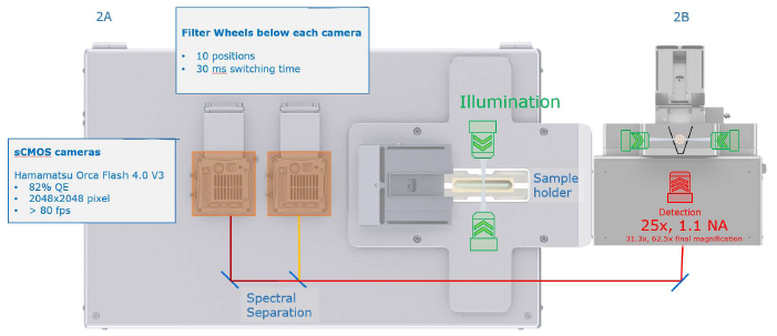
a.   The Bruker TruLive3D is a dual sided illumination light sheet microscope. The dual light sheet is projected on the sample by a pair of water immersion 10X 0.3NA microscope objectives. The detection objective is a water immersion 25X 1.1NA objective. An additional magnification changer can be added for a resulting 31.3X and 62.5X. This allows for a resolution down to 255nm in xy.

The images are acquired on two Orca Flash 4.0 cameras. Each camera has a motorized filter wheel on its path. Through a combination of dichroics and filters the long wavelengths are directed to one camera (the horizontal one) and the short wavelengths to the other (the vertical one).

b.   On the back of the microscope you will find the laser stack on the table, the 4 laser lines are launched in an optical fiber plugged into the microscope. The gas mixer and humidifer is found right next to the microscope. In case the water level in the column is low, refill using sterile DI water only. The green line is for the CO2, the blue for the air and the yellow line for nitrogen in case someone needs it. The gas mixer controller is the black box located on top of the white temperature controller. On the right is the microscope system power supply. In case of emergency, turn off everything with the big red button.

The figure below is a schematics from Bruker showing how the sample is imaged by the Light-Sheet. Your sample should be sitting at the bottom of the little cuvettes that have to be used as sample holders.

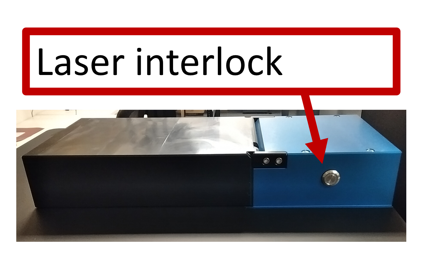
c.   Every time you open the sample chamber the lasers will turn off automatically. When you close the lid, always remember to press the interlock button on the back of the sample chamber.

d.   When you open the sample chamber, you will see a lens on the lid. This is for illumination with an LED light, directly above the sample. It is used to find the sample. In the sample chamber you will see the detection objective at the bottom and the illumination objectives on the sides. The sample will be held in the metal brackets that are attached to the translation stage.

A more comprehensive schematic of the sample chamber can be found on the Bruker TruLive3D manual accessible on the Luxendo computer and is reproduced here:

e.   The translation stages can be controlled with the Luxendo software or with the space mouse. The Z direction is up and down in the direction of the detection objective. X is the direction along the sample and Y is the direction across the sample, along the illumination path.

3. Bruker TruLive3D Lux-Bundle overview

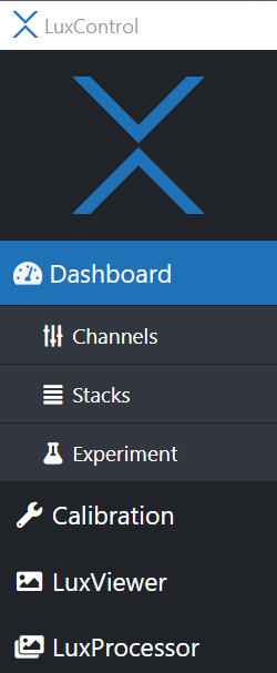
1. Once the microscope, cameras and temperature controller and gas mixer are on it is time to open the LuxBundle software. Find the Luxendo logo on the taskbar and click on it.

If you are using the temperature controller the water bath in the chamber will heat up and create condensation on the lid which would then drip on your sample. The lid heating should turn on automatically but always check that it is ON. 

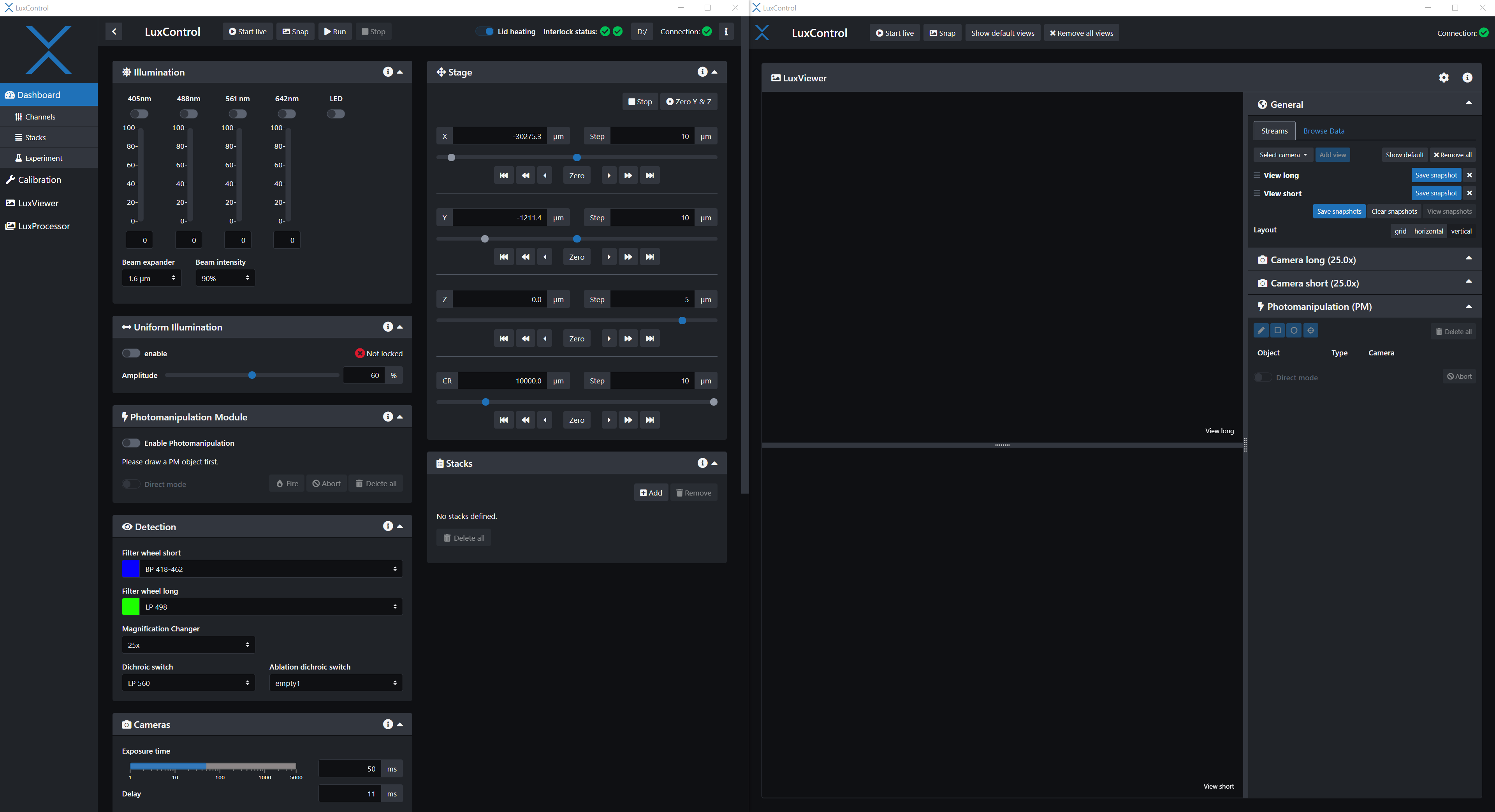
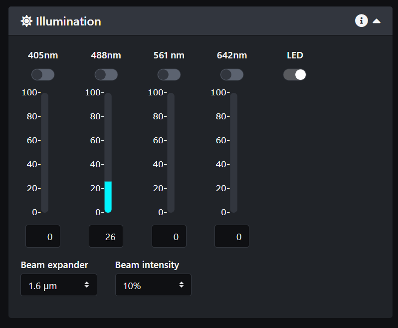
The illumination panel has the 4 different laser lines and the LED option. The beam intensity can be controlled between 10% or 90%. The beam expander controls the NA of the illumination objectives. This will have an effect on the characteristics of the Light Sheet.

The Stage panel allows you to control the translation stages, the focus of the detection objective and it correction ring.

The detection panel is where you will set the emission filters for the different channels (short wavelengths and long wavelengths). You can also change the magnification there and the dichroic switch between the two cameras. There is also an option for the ablation dichroic switch in case you are planning to use the photo-manipulation feature.

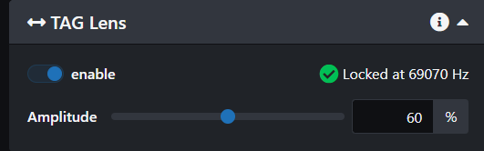
The TAG lens panel allows you to enable the TAG lens function which makes the light sheet longer.

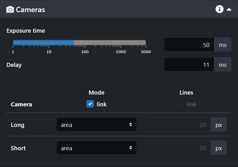
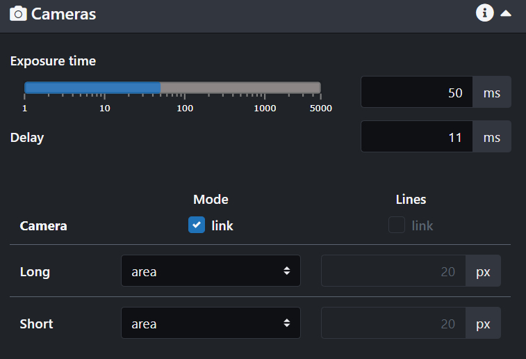
The camera panel is where you can control the cameras, their exposure time and delay. You can switch between line and area mode. In Line mode you can use a delay of 1ms but in area mode you should always have at least 11ms.

You can also unlink the cameras there and turn one off if you need.

Last we have the PM panel that has the photo-manipulation functions. You will learn more about this in a later page.

4. Bruker Trulive3D calibration

Calibration of the laser beams is critical for optimal imaging and should be done prior to every experiment.

If you are using the temperature controller you should wait that the temperature in the sample chamber is close to the set value to perform the calibration as temperature is one of the main factors that can change the beams alignment.

NOTE: We found that it is best to install the sample in the sample chamber and let it sit a little bit before performing the calibration. The calibration is done in the water under the sample. Having the sample already in place prevents any changes in temperature when opening the chamber to install the sample.

Install the sample in the sample holder and into the sample chamber. Hold it at one end and push the other end against the end o the brackets then press the other end into place.

On the left side click on the Calibration tab.

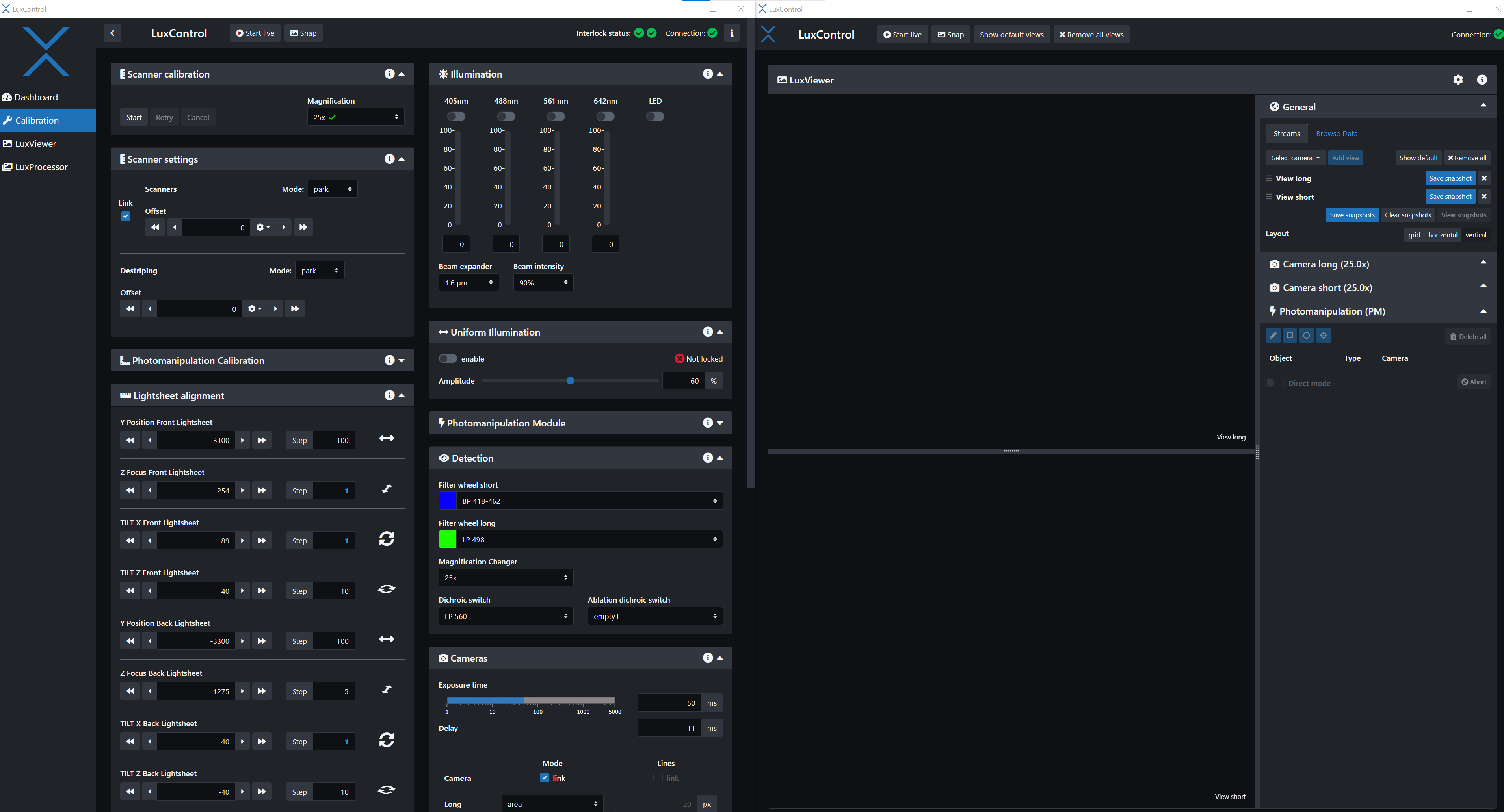
Below is a view of the calibration page as it first appears.

To observe the beams and align them you want to have water in the sample chamber. You can turn on any of the laser lines but in pure water, only the 488nm laser will produce enough scattering to be observed. 

Select the beam intensity at 90% and turn on the 488nm laser to about 50% or above.

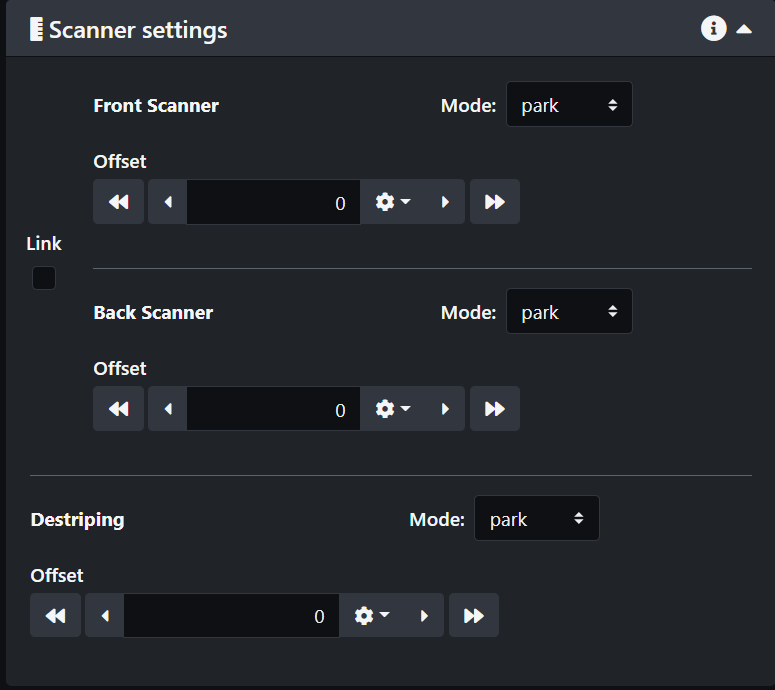
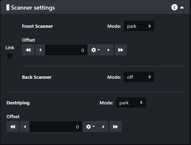
The next thing you need to do is to unlink the scanners so you can control the beams separately. Select the option "park" for both beams and check the camera display.

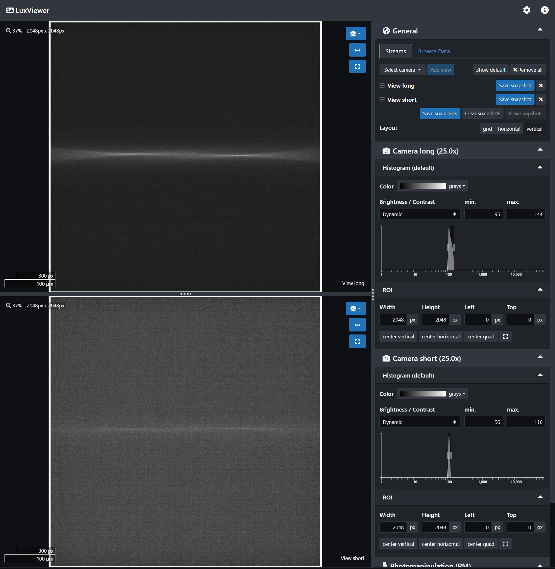
When both cameras are connected you will see the same image from two different angles. The beams may look fuzzy and not in line as in the image below. If they are too dim, try increasing the laser power or the camera exposure time. They may also be far out of focus.

Calibration is better done one beam at a time. Start with the front scanner and then repeat for the back scanner. Go in the scanner settings and select "off" for the back scanner.

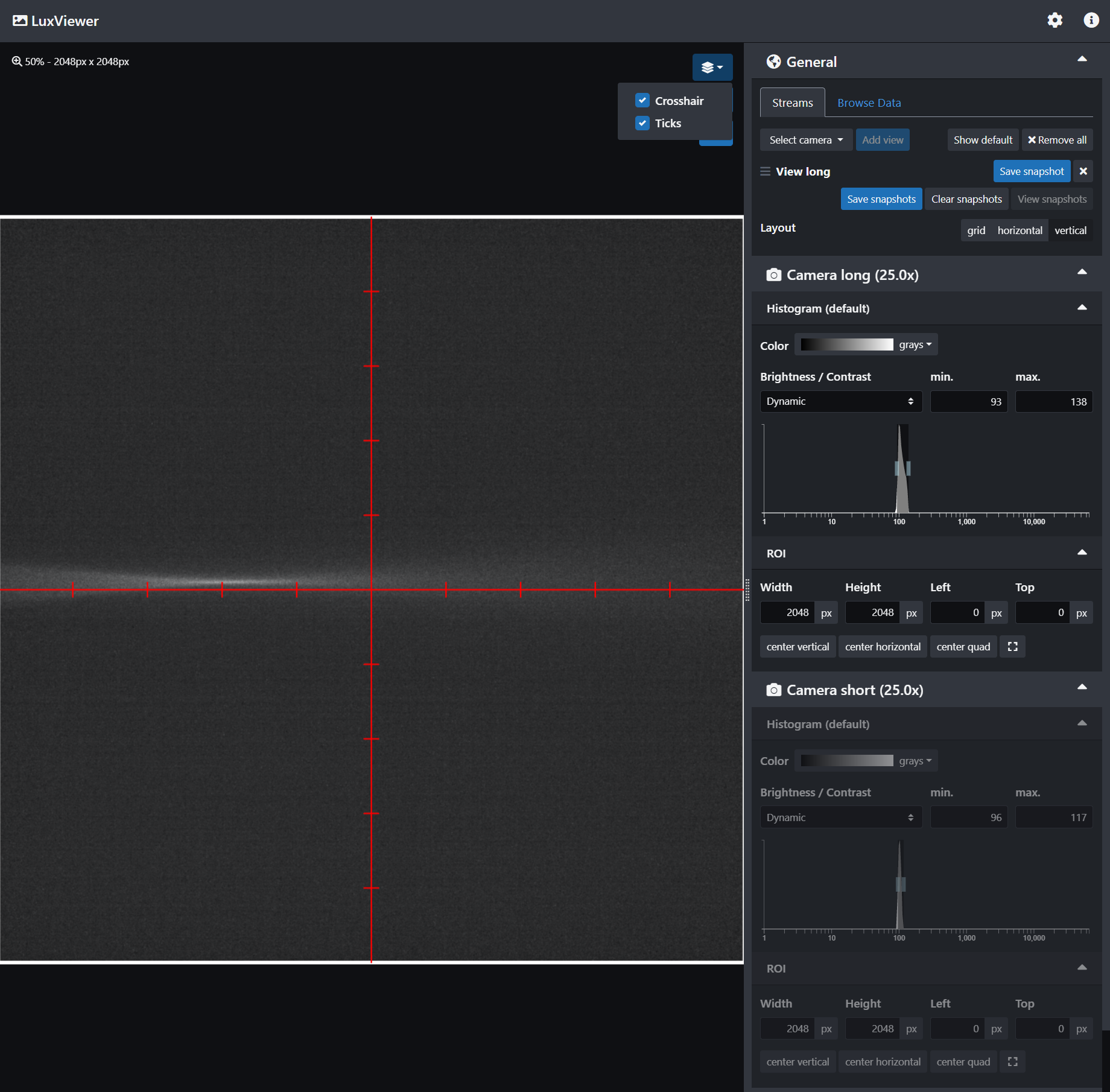
Now only the front beam will be displayed. In order to align it you can use the Crosshair and Ticks markers. You also don't need to have both cameras connected, it makes it easier to have only one image displayed. On the screenshot below, the beam is slightly offset with respect to the crosshair and not very sharp. You will want the beam to be uniformly centered on the line and the center of the beam aligned with the second tick from the center, at least for most experiments.

Offset correction: Go in the scanner settings and change the offset value until the beam is perfectly aligned with the crosshair. It usually requires small values between 0 and 0.1. Once you are satisfied with the result click on the store button next to the offset value. This will save the value through the experiment.

Z focus adjustment: In the stage control, select the Z Front Lightsheet and adjust the value until the beam is as crisp as possible with a narrow waist.

Y position adjustment: In the stage control, select the Y Front Lightsheet and adjust the value until the middle of the beam is on the second tick from center.

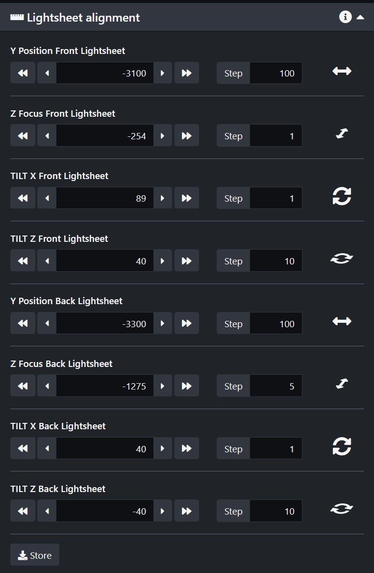
The last two parameters to adjust are the In-plane tilt "Tilt X Front Lightsheet" and Out-of-plane tilt "Tilt Z Front Lightsheet". To better visualize them you can turn the TAG Lens on.

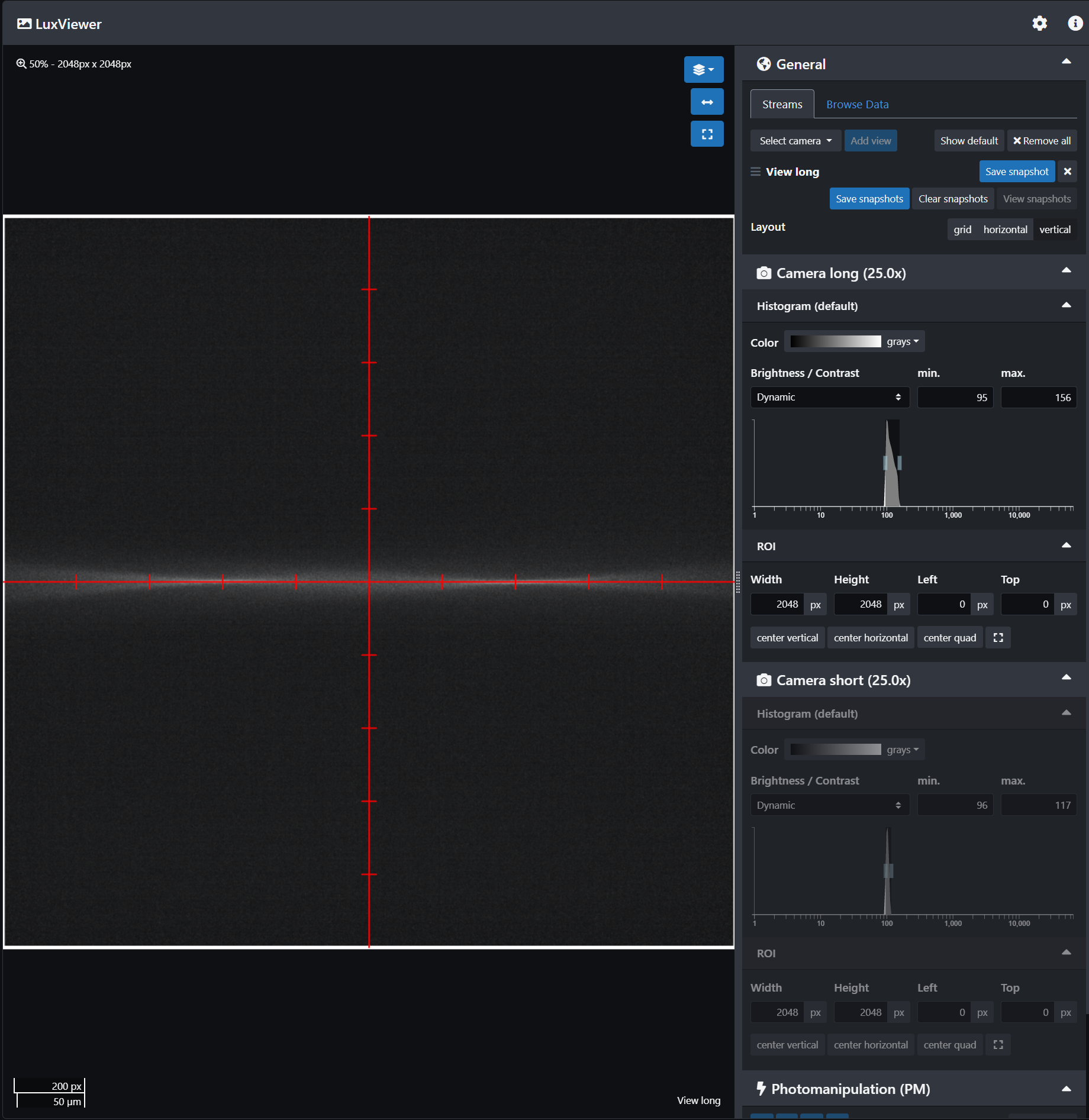
In-plane tilt adjustment "Tilt X": Change the value until the beam is perfectly centered along the crosshair.

Out-of-plane tilt adjustment "Tilt Z": you want to observe a uniform thickness of the beam along the crosshair. Change the value until it looks the most uniform.

Store all the values by clicking on the save button at the bottom of the Lightsheet alignment panel.

Repeat the process for the back scanner. Turn the front scanner off and park the back scanner then adjust the offset, the Z, Y, In-plane tilt and Out-of-plane tilt. Remember to turn off the TAG lens to start the procedure and turn it back on the adjust the in-plane tilt and out-of-plane tilt. Save your values and park both beams to check they are both well aligned.

The last step of the basic calibration process is to perform the Scanner Calibration.

Make sure both cameras are connected. Then click start and click on the next steps until the calibration is finished. Click Finish and if successful you are good to go!

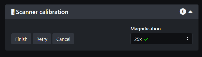
NOTE 1: If you are planning to use more than one magnification you should repeat the scanner calibration for each magnification.

NOTE 2: If you need to perform photo-manipulation you will need to calibrate the PM module as well. Instructions will be detailed in the Photo-Manipulation page.

 

 

Cameras alignment

 

In the event that the short camera is shifted with respect to the long camera, we can correct for it.

• Use a sample with features stained for long wavelengths emission and short wavelengths emissions. Beads are ideal for this.
• Check that the beads are in focus on both cameras. If one channel looks slightly out of focus, use the "camera alignment" tab in the calibration panel to adjust the focus.
• Center one bead exactly at the center of the cross-hair marker on the long camera.
• Use an allen key from the Bruker tool kit to manually adjust the short camera using the knobs at the base of it until the same bead is centered on the short camera too.

5. Bruker TruLive3D Finding the sample

Make sure you performed the calibration of the system before lowering your sample in the chamber.

1. Finding your sample

• You should have already installed your sample, so the first step is to lower the z stage to bring the sample between the two illumination objectives. 
• You can also use the space mouse to move the dish to its position above the detection objective.
• Click on Dashboard in LuxBundle.

         

• In the illumination panel, turn on the LED light. Then click Start Live.

  

   

   

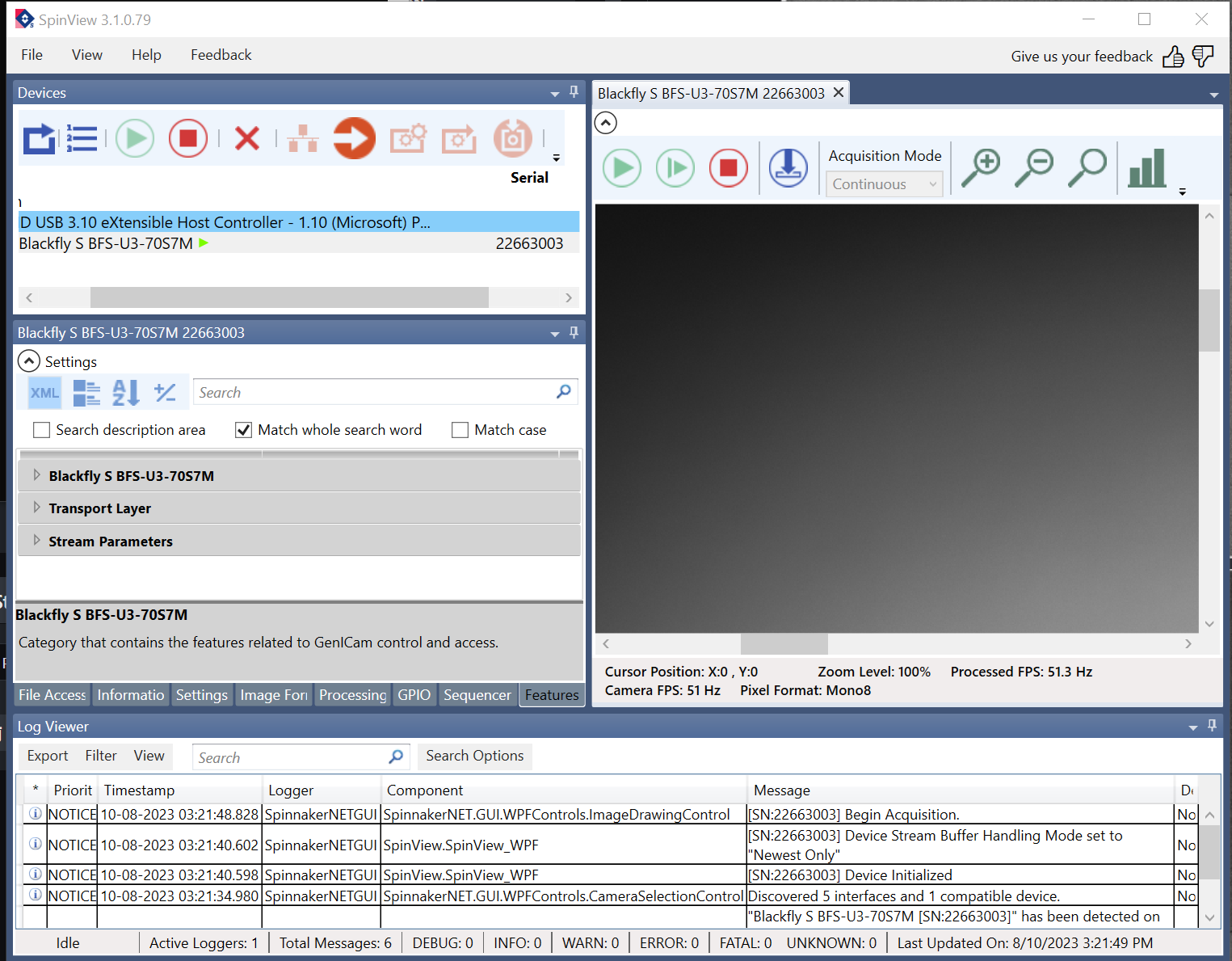
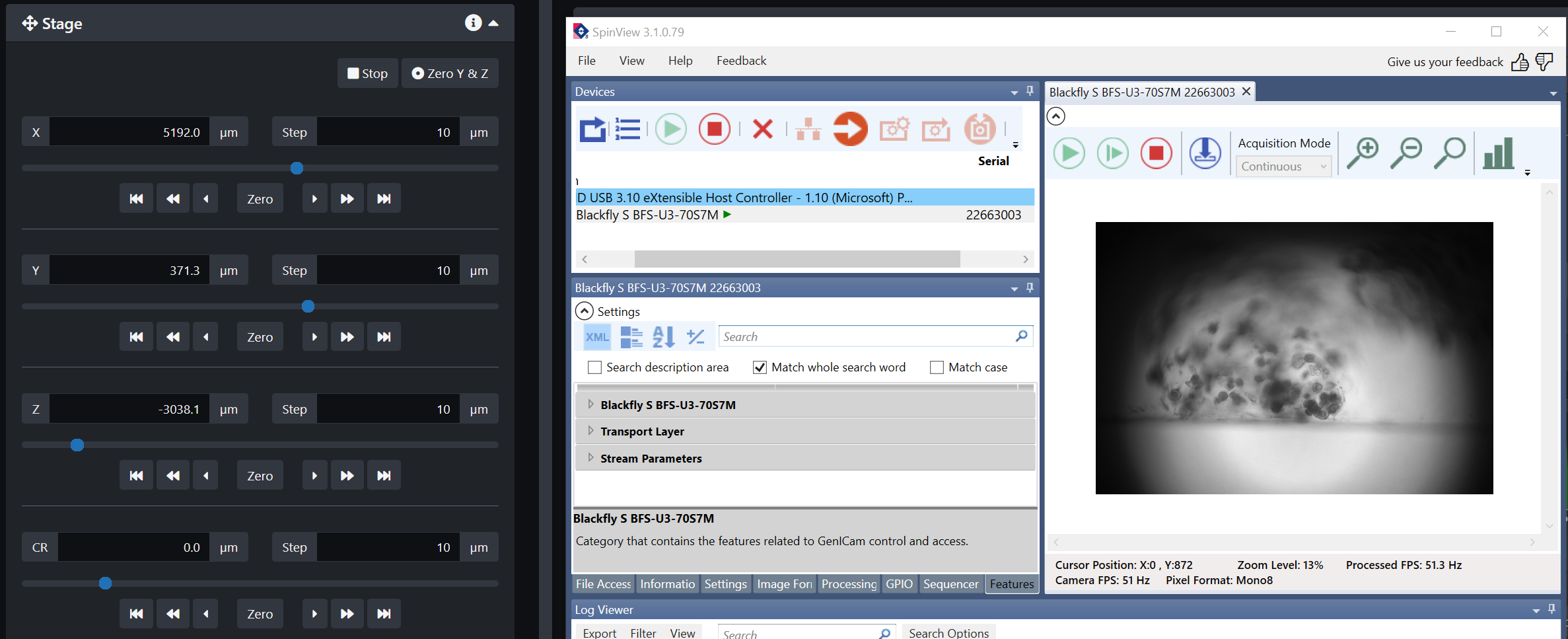
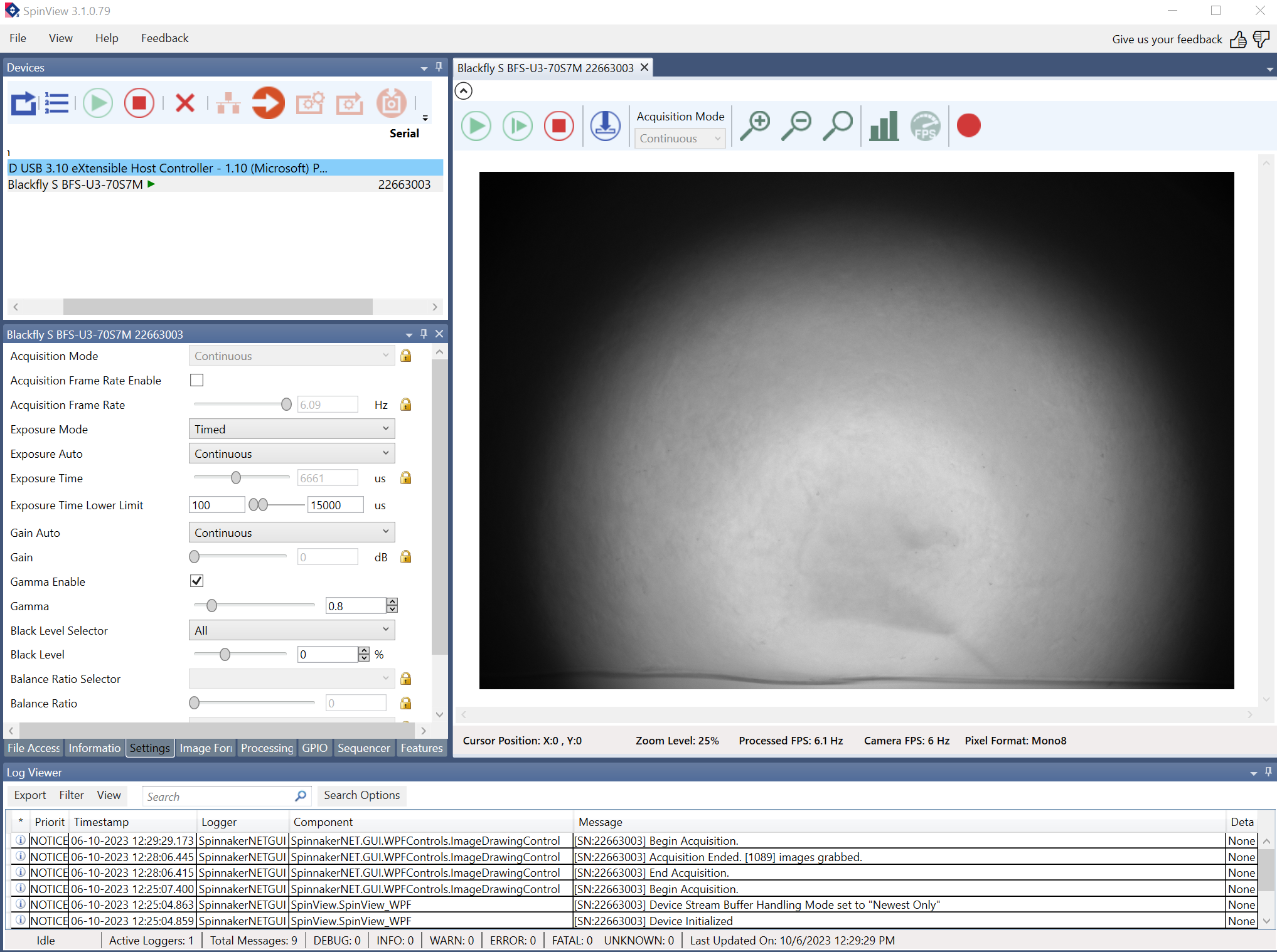
• Open the SpinView software and select the Blackfly camera then click the green arrow. There is a small camera in the system that looks through one of the illumination objectives. 
• Click on the image area and scroll out to see the entire field of view

  
  

  
• Go back to LuxBundle and use the stage control buttons to move the sample until it appears in the field of view of the Blackfly camera.
• If your sample is already above the detection objective, move the Z stage to lower it. 
• If it is not above the detection objective, move the X stage as well.
• Move the Y stage to bring it in focus and confirm that what you are looking at looks like what you expect and is not an artifact. 

NOTE: This is not the focus of the detection objective! It brings the sample in focus for the illumination objective the Blackfly camera is looking through. This step is for identification only.

• Now that you know the sample is in the right location, turn off the Blackfly camera by clicking on the red square and turn off the LED light in LuxBundle.
• Select the laser lines you need for your sample.

• Select the emission filters for each camera. If you are not sure which filters to select for your sample please refer to page Bruker TruLive3D emission filters and fluorophores spectrum and try to pick a pair of filters that prevents any overlap in emission. 

• Connect both cameras and start live

• Adjust the camera exposure and select either line mode or area mode. Line mode rejects more background but for sample finding it is best to use area mode. If you only need one camera, unlink the camera and turn one off.
  • Area mode to find the sample

• • Line mode for imaging

• Turn on the TAG lens for a little better image quality:

• Find a location of interest in the sample using the stage controls. Scroll the z slider to find the limits of your z-stack.

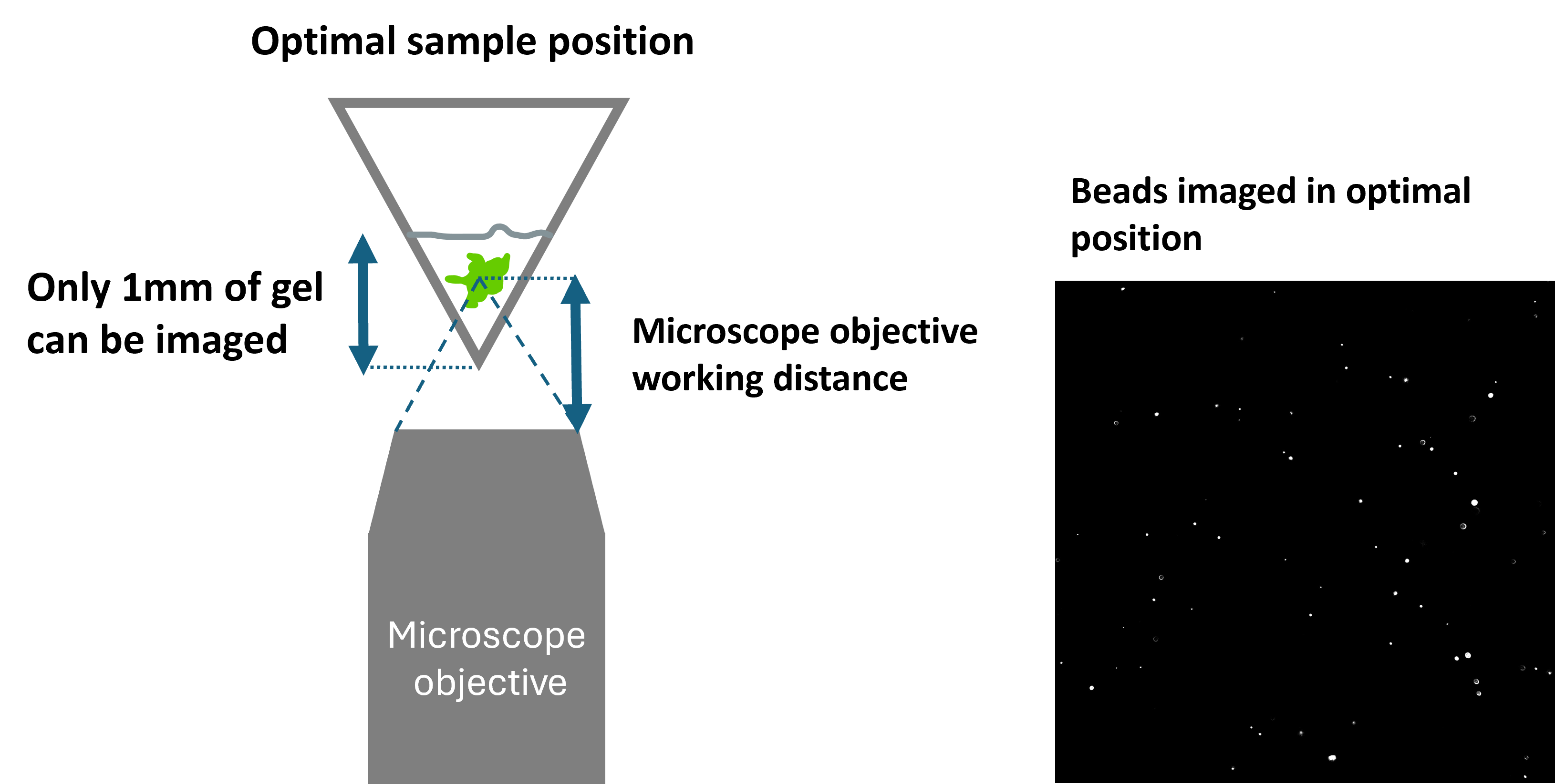
To acquire the best images from your sample, you need to look at areas that are in the middle of the dish, within the layer of gel that can be imaged. Only the lower 1mm layer of gel at the bottom of the cuvette can be imaged. If your sample is sitting above this, you will not be able to image it. 

The detection objective is fixed, when you move the z stage your are moving the sample dish up and down. The biggest z-stack you  can acquire is around 1mm, that is if you start below the dish and go as far as the working distance of the objective goes. 

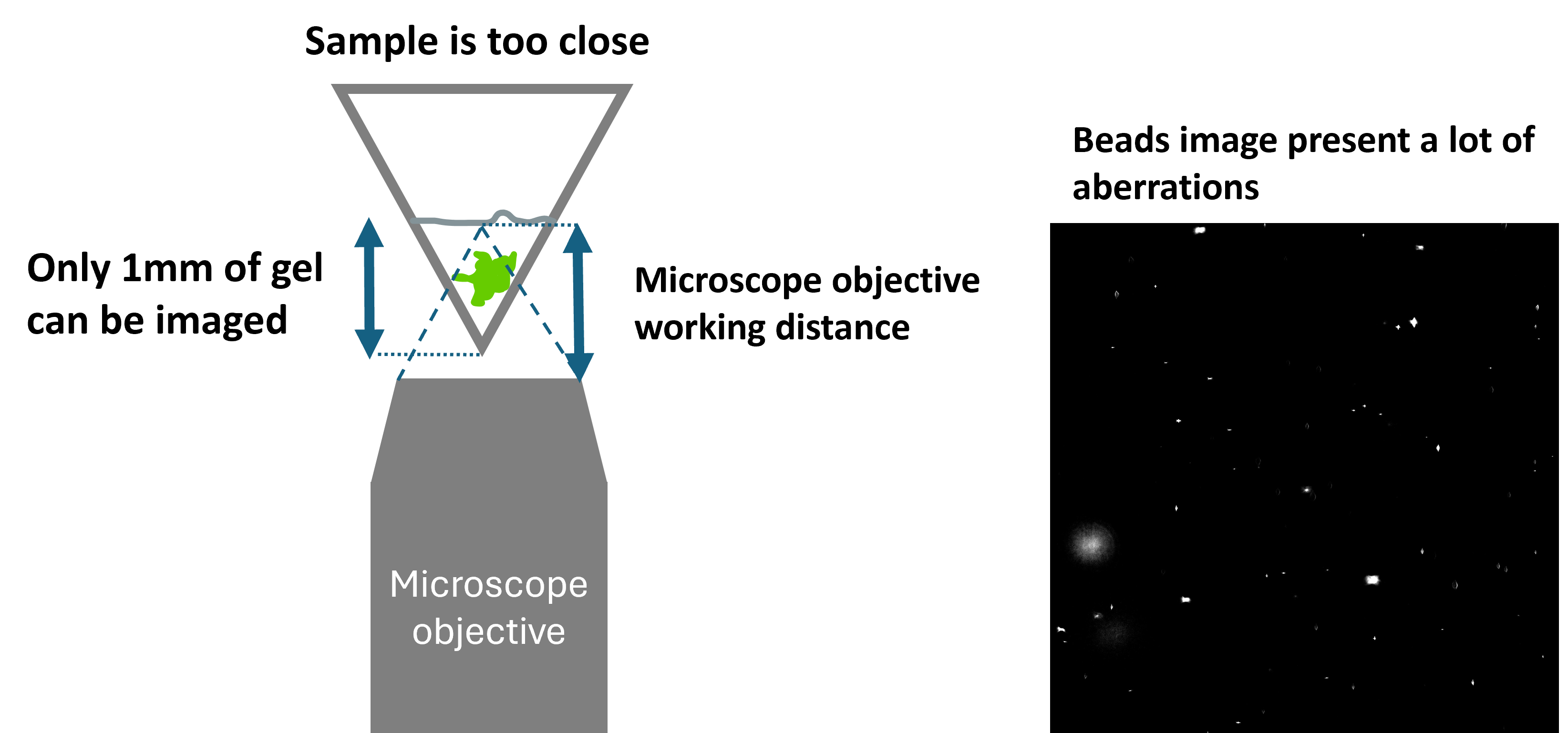
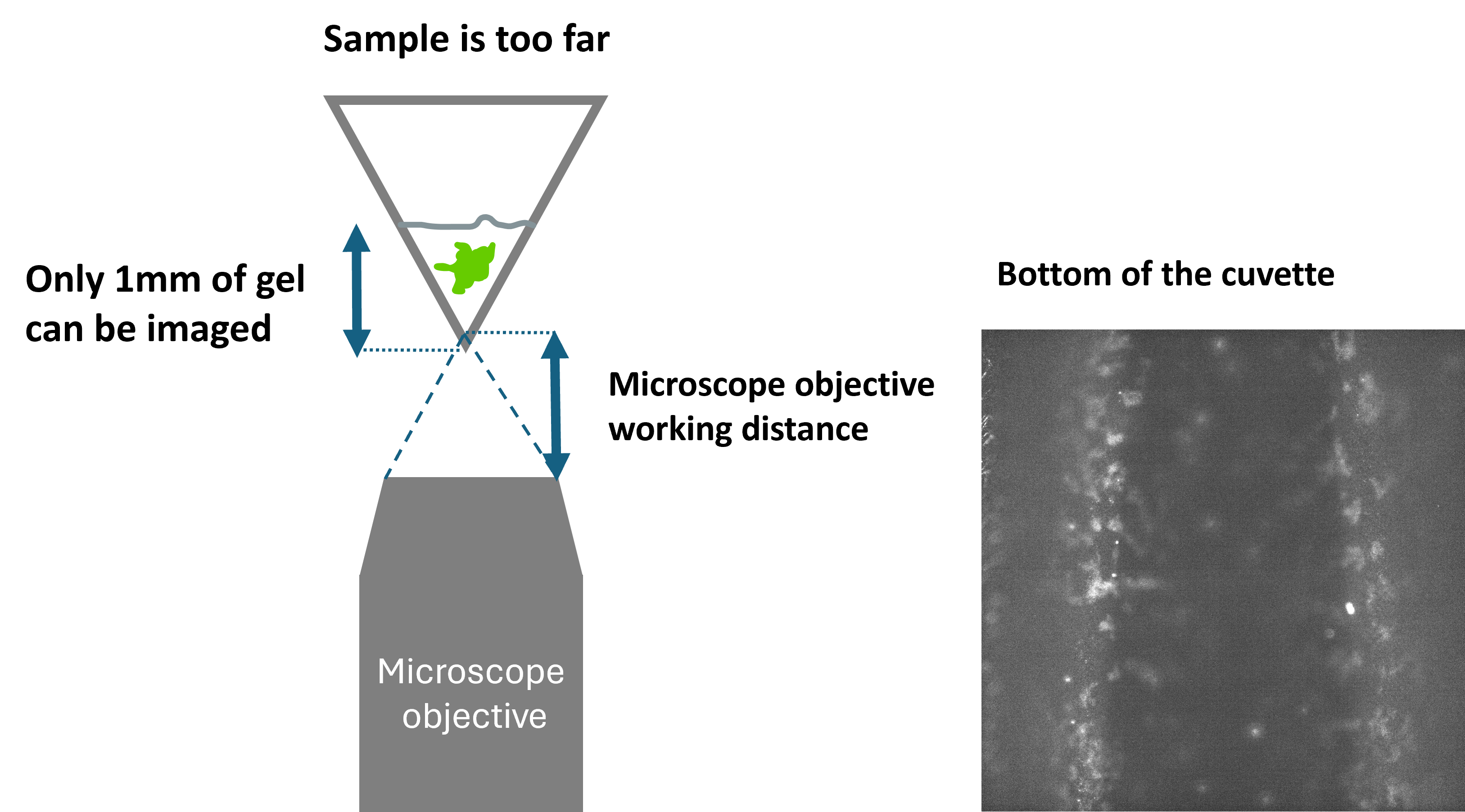
The working distance of the objective is what defines your imaging range. However, the images acquired at the limits of this range will not be ideal. If the dish is too high above the detection objective you will be looking at the bottom of the cuvette. If the sample dish is too close from the detection objective, you will be looking far into the gel and this will generate more aberrations.

If you are looking at the edges of the dish, you will also get more aberrations.

The following figures show how to best position the sample and the resulting images with a bead sample.

• Optimal sample position

• Sample is too close, more aberrations are present due to the thick layer of gel

• Sample is too far, we look at the bottom of the dish

• Stage coupling to the correction ring to reduce spherical aberration

The LuxBundle software now has the option to perform stage coupling. We can use this feature to couple the z stage with the CR stage (Correction Ring) and optimize spherical aberration correction throughout the entire z-stack. This step should be done once at the working temperature after calibrating the system. We need to use the beads sample for this as beads are the most appropriate object to identify aberrations and correct for them.

Below are the steps to achieve ideal coupling, along with the values used to couple the Z stage and the CR stage at room temperature and 37C. The stage coupling will be discussing and practiced in your training but you can re-use the values presented in this wiki for room temperature or 37C when you introduce a new sample.

• • Stage coupling panel in the Calibration tab:
    
  • Once you have your beads in the FOV, select a Z position and manually adjust the CR until the beads look as sharp as possible and spherical aberration seems to be minimized. It is a good idea to go over the whole Z range and pick a position close to each extremity but not the last position you can possibly pick on each side.

• • Once the Z stage is coupled with the CR stage, click Add to couple your current Z position with your current CR position. This will be one end of your range.

• • Then go to another position in Z and optimize the CR value to minimize spherical aberrations. Click Add stage positions to add the new values.

You now have 2 values for stage coupling and the CR stage will extrapolate values to best fit the entire Z range you selected. Below is an overview of the calibration panel with the stage coupling values set for room temperature.

• • Back in the Dashboard, click Enable Stage Coupling to have the CR stage move along the Z stage when imaging
•  
  • Values you can use for ROOM TEMPERATURE stage coupling (simply copy those values in the Calibration stage coupling set-up):
    • • Z = -2347   CR = 700
      • Z = -3014   CR = 1405
  • Values you can use for 37C TEMPERATURE stage coupling (simply copy those values in the Calibration stage coupling set-up):
    • • Z = -2347   CR = 600
      • Z = -3014   CR = 1225

• Further tips on how to use the correction ring:
  • Find the center of your z-stack and look for circular features that appear to be in focus. If they have a little bit of a halo despite being the most in focus in this z-plane then try changing the correction ring to see if the halo disappears. If this is hard to see, try to get the best looking image of your sample in terms of sharpness.
  • Go to the beginning of the z-stack and find a circular feature that is in focus. Try changing the CR value to see if it makes it better. Repeat at the end of the z-stack.
  • To adjust the CR during an experiment you can make it change over the length of your z-stack after selecting the values that improve the image best at the beginning and the end of the stack. However, this is a little bit arbitrary and the CR value may not be optimal for each z-plane. In doubt, I recommend adjusting the CR value for the center plane of your z-stack and leaving it the same. 

6. Bruker TruLive3D Experiment

This page will guide through the steps to set-up a basic experiment.

1. Setting up an experiment

You have many possibilities to set-up an experiment with the Bruker TruLive3D. You can record a single z-stack at several time points, multiple z-stacks at several time points and you can also acquire bigger areas than the field of view by tiling the images together.

You can acquire data in a single channel with one or multiple laser lines on and simultaneously acquire images for two different emission channels, or you can create several channels for each laser line.

NOTE: if you only need one camera to acquire your images make sure you turn off the other one in the camera panel (unlink them and turn one off) otherwise both cameras will capture images which doubles the size of your data. 

CHANNEL:

• Create a channel. This will have all the current savings on the screen: laser lines and power, beam expander setting, detection filters, camera settings. If you change a setting, remember to update the channel. 

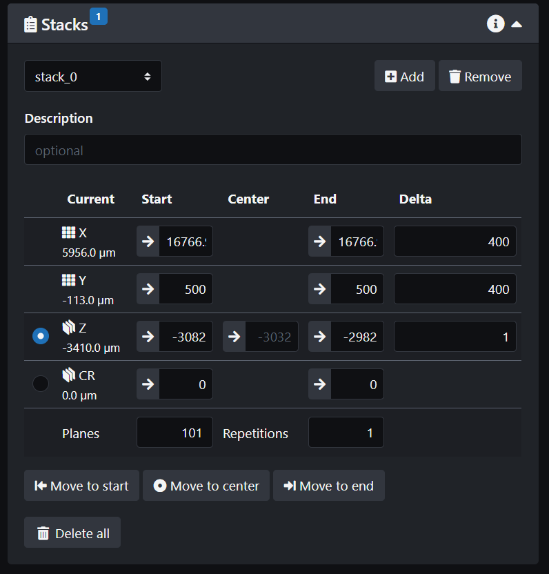
Z-STACK:

• Create a z-stack. Move the Z stage until you find the stack you want. At the bottom of the stack, click on the arrow in the z-stack parameter to update the value read on the stage control panel. Then go to the top of the stack and repeat the process. To visualize the data, the z-stack panel has buttons to go directly to the middle, bottom or top of the stack.

EVENT and TASKS:

• Create an event. This will open two other panels with tasks and trigger. Set up your task(s) with the channel(s) you want and the z-stack(s) you want. You can have the same channel for all the different z-stacks or different channels with different z-stacks.

TRIGGER:

• Set-up your trigger. This defines the parameters for the timelapse. 

SAVE YOUR SETTINGS:

• Select where you want to save your data. If you are saving your data locally, create a folder for your Group in the Disk D and select this folder. 
• Follow the procedure taped on the wall to name your data: Lab_Initials_Date_DataDetails
• ALWAYS save your settings for future use. Make sure you save those settings in your folder.
• If you are saving directly on your server select it as a location. We do not recommend this though as the connection may drop during acquisition. To be able to save directly on your server you must ask the Beckman Center admin to set it up. 

• Click Run when everything is ready! 
• When you experiment is done please refer to the Data management page to follow the procedure to transfer and delete it.
  

LuxBundle saving process:

• • LuxBundle creates a new experiment folder in the folder where you save your data. This folder has a specific timestamp following this convention: year_month_day_hoursminuteseconds. For example, if an acquisition is launched on December 13, 2023 at 3:19:26pm then the timestamp will be 2023_12_13_151926. 
  • Inside the timestamp folder, sub-folders are created for each stack and channel combination. The folders are named stack_(n)_channel_(n). For example, if you acquire 3 z-stacks with a single channel you will have 3 sub-folders named stack_0_channel_0, stack_1_channel_0, stack_2_channel_0.
  • If you acquired tiled montage acquisitions, the stack sub-folders will include the X and Y coordinates of each tile position such as stack_0_x00_y00_channel_0,  stack_0_x00_y01_channel_0 and so on. 
  •  Within each sub-folder, the image data for each stack is written as Cam_Long_00000.h5 and Cam_Short_00000.h5 files. For time series, the h5 files include the time points such as Cam_Long_00001.h5 and Cam_Long_00002.h5 etc. The h5 files can be opened in FIJI, they are open source format. 
  • LuxBundle also creates files that contain the metadata for each experiment. Those are the JSON files that can be opened in Notepad. They contain the microscope settings.

SPECIAL CASES:

• When you set an experiment with several events and stacks of different sizes with different timepoints (triggers), the data will save properly but the bdv and ims header files will not write properly. When you see an error message telling you this, you know that you will need to post-process the data to generate those header files. This can be done in the Image Processor and is explained below. Follow the instructions to create separate ims and bdv header files. Make sure you process each stack separately as a different task.

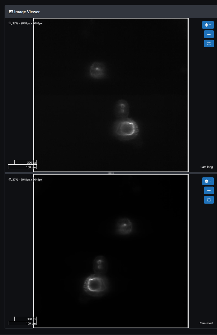
         2.  Visualize your data

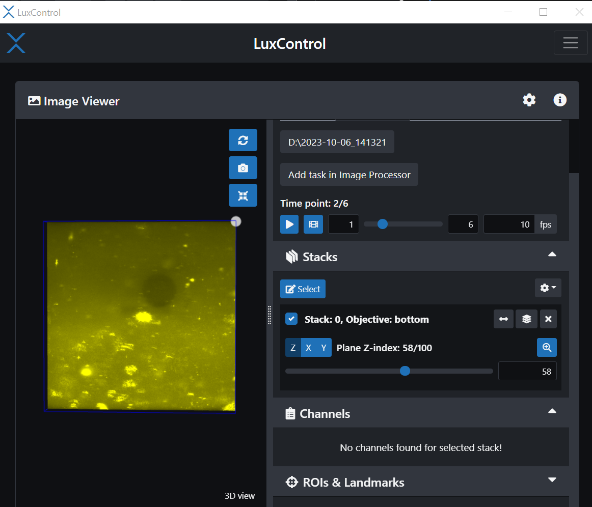
• Click on image viewer

The image viewer in LuxBundle allows you to visualize the data frame by frame. It is not a 3D viewer, unlike Imaris viewer, but can give you an idea of what happened during your experiment at each time point. You can also play a movie of the z-stack. When you open the image viewer you can select the image data you want.

3. Process the data

Finally, LuxBundle has an image processor function that allows you to do a few things to process your data. Click on the LuxProcessor tab.

For a complete overview of the capabilities of the Image Processor, please read the User Guide located in the little book icon on the top right corner of the LuxControl window.

When your data is acquired, it automatically creates an imaris (.ims) header file along the Fiji Big Data viewer (bdv.h5) header files. However, depending on the size of your data set loading the images in imaris can take a very long time.

It also creates an ims folder where you can find the ims headers for the different stacks you acquired. The raw folder contains the raw data.

NOTE: As of May 2024, the ims headers created display the channels in opposite orientation making it impossible to visualize the two superimposed.

The image processor enables you to process your data stack by stack and create separate imaris header files. It also creates a mip folder with the maximum intensity projection of each stack. This can be useful in some cases to gather a quick view of the experiment and see if it looks good.

Here, we will guide you through the steps to perform this task. For more information and potential debugging please refer to the User Guide in LuxBundle. You can also download the PDF version to read offline. And always ask the Beckman Center staff for guidance or in doubt!

• Add a new Task in the Tasks panel
  
  
  
  
• In the Task Configuration panel Name your new task and then click on Input.
  

• Browse through your data to select the image folder that you would like to process.
  

• If you only want to process a few stacks then de-select the ones you don't want.
  

• Click on the Registration tab and turn it off.
  

• Click on the Fusion tab and turn it on. You don't need to change any settings here.
  

• Click on the Output tab and select "Separate" on the "Bounding boxes" option. Width and Height of 1 will be full resolution images. If you want this processing step to go faster and you are willing to low some image quality you can down sample by choosing Width/Height greater than 1 and Depth greater than 1 as well.
  

BigTIFF: If you want to save your data as TIFF files, check the box for "Copy images to BigTIFF".

• The next step is to run the Task. Go back to the Tasks panel and scroll to the right then click on the arrow and click run. You can also stop or delete the task in this menu.
  

• IMPORTANT: if you want to have a separate processed folder for each stack, simply process the stacks separately. Create one task for each stack and then click "run all" to process all the stacks in one go.

• When you go to your image folder you will now see a "processed" folder that contains the separate imaris headers and the task configuration parameters as a JSON file. It also contains the mip folder.

7. Bruker TruLive3D Data management

Data acquired on the Bruker TrLive3D will typically be very large, on the order of TeraBytes of data. The Luxendo computer has enough internal capacity to store up to ~20TB of data. This seems like a lot of storage but we are asking the users to transfer their data to their own server/storage devices immediately after an experiment so that there is always a lot of space for the next user to save their experiment.

Data management is going to be a major challenge for working with the Bruker TruLive3D Light-sheet microscope. Please read this page carefully and plan accordingly.

Data acquisition

Option 1: Write your data locally on the Luxendo computer. This is the recommended safest option.​

• Update the Bruker Data management Book Keeping excel sheet with your experiment settings

• Update your own excel sheet with your experiment settings. You can use this template.​

• Create a folder for your group in the DATA drive. ​

• Save your data in this folder with this nomenclature: Lab_Initials_Date_DataDetails for example Anseth_KA_20230719_organoidsDay3​

• Once the experiment is done, transfer the data to your network drive or to an external hard drive.

• MAKE SURE YOU SAVE THE EXPERIMENT SETTINGS!!!​

• Delete your data from the computer.​

• Data that has not been deleted within 30 days will be deleted by facility staff. If space is needed for another experiment, facility staff will reserve the right to delete data without warnings.

Option 2: Write your data directly on your network drive. This may work for short experiments and save you the transfer process. Unfortunately, the internet is not always reliable, to avoid any interruption during a long experiment over several hours we recommend writing data on the Luxendo computer. ​

• Update the Bruker Data management Book Keeping excel sheet with your experiment settings

• Update your own excel sheet with your experiment settings. You can use this template.​

• Save your data with this nomenclature: Lab_Initials_Date_DataDetails, for example Anseth_KA_20230719_organoidsDay3

• MAKE SURE YOU SAVE THE EXPERIMENT SETTINGS!!!​

In doubt always check with facility staff about how and where you should save your data.

Data pipeline

The following diagram is the vision for future data pipeline in the Beckman Lab:

• Acquire data on Bruker computer
• Perform any kind of processing you want with the LuxBundle software
• Transfer your data to your server via the 10GB ethernet line, or to your personal hard drive storage

• Analyze your data with the Imaris workstation which will be installed next to it, with a hard wire connection.
• Transfer your data to your server via the 10GB ethernet line, or to your personal hard drive storage

8. Bruker TruLive3D Using the photo-manipulation (PM) feature

The Bruker TruLive3D has a photo-manipulation (PM) feature that you can use to ablate specific areas of your sample.

Calibration of the PM module

Before performing any kind of photo-manipulation, the PM module needs to be calibrated. 

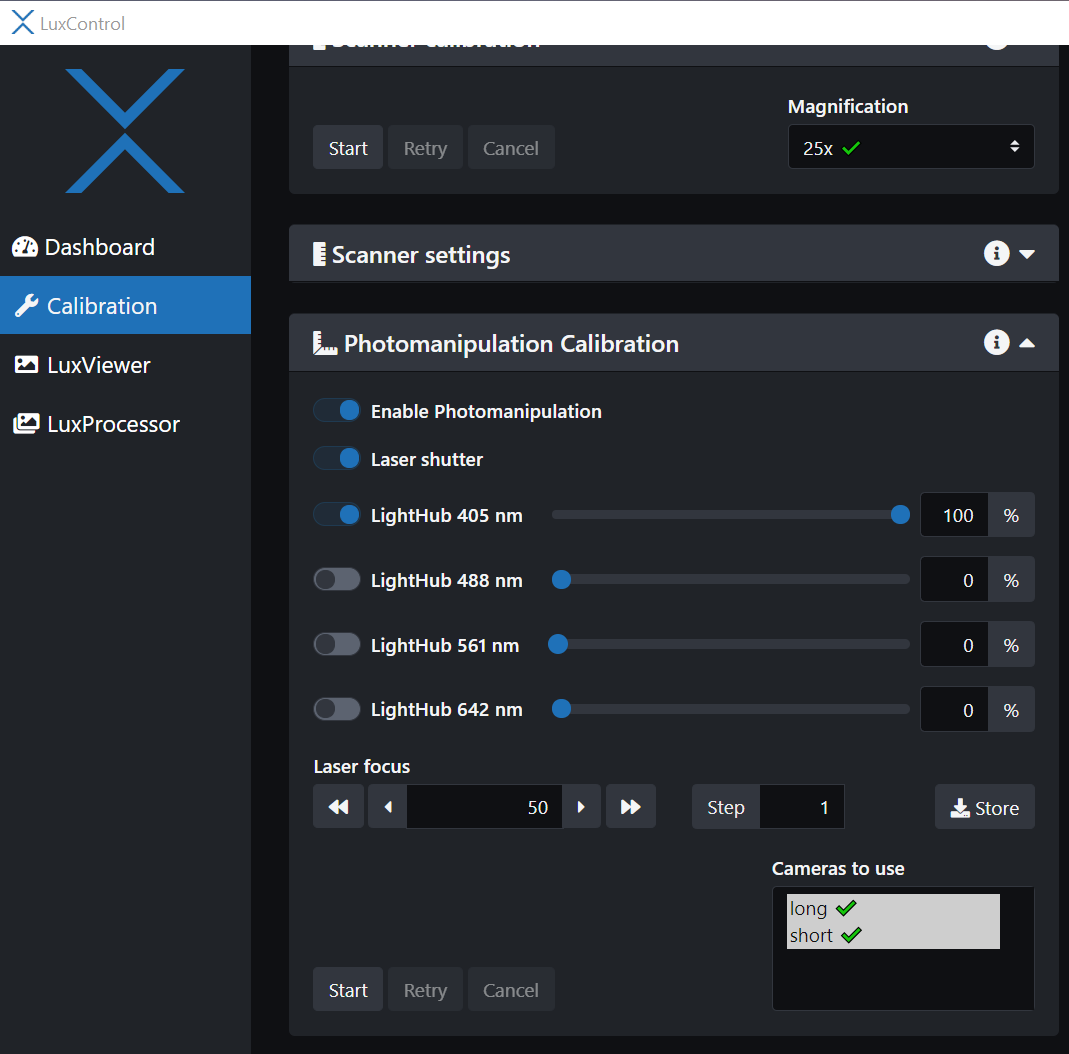
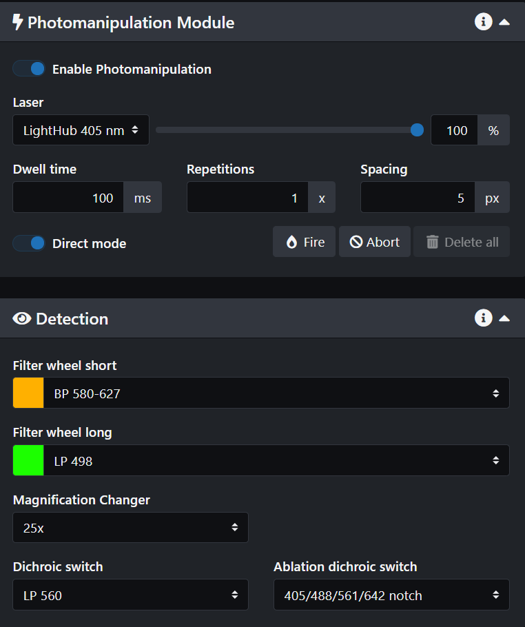
Click on the Calibration tab and open the Photomanipulation Calibration panel:

• Enable Photomanipulation
• Laser Shutter
• LightHub 405 nm on, with up to 100% intensity
• Select which camera to use, if you are not sure you can select both and the calibration will be done for both of them. You need to click on them to highlight them, as shown below.

• Start live and select the correct filters to observe the laser spot. For the 405nm laser, the BP 418-462 for the Filter Wheel Short and the LP 498 for the Filter Wheel Long usually work fine. 
• Make sure to select the Ablation dichroic switch!

• Start the cameras Live, you should see a bright spot at the center of the field of view. Adjust the Laser focus in the Photomanipulation calibration panel until the spot is sharp and bright.

  

• If the spot looks too dim you can increase the camera exposure time.

• 
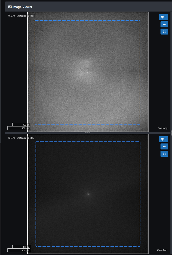
• There is 5 steps in the Photomanipulation Calibration. If they all calibrate well you should see the laser spot move in 5 different location starting with the center and the purple circle should follow the laser spot.
• When you have successfully performed the 5 steps click finish. The PM module is now calibrated!
• If you need to perform photomanipulation with a different laser, just select another line and repeat the steps. You will need to change the filters and adjust the camera exposure as the other laser lines are less visible in the water due to less scattering.

• Troubleshooting

  • If the calibration does not succeed it is usually because the laser spot is too dim. Try adjusting the parameters until you can see the spot better: change the laser intensity, filters, camera exposure, double check you optimized the focus of the laser spot.
  • If you know you only need to perform the calibration on one camera because you will only image one fluorescent wavelength, you can select only the appropriate camera and start the calibration again. It is usually easier to calibrate the short wavelengths camera.

Define the PM event

The next step is to define the photomanipulation event in your sample. 

• Locate your sample with the BlackFly camera. In this tutorial we used a simple fluorescent gel, there is no bio sample in it. Turn on the LED light and open the SpinView software. Click Live.

• Once your sample is centered above the detection objective, close the BlackFly camera and start live in LuxBundle. Turn on the laser line(s) you need for your sample. Find an area you want to ablate. In the following example we are looking at a fluorescent gel.

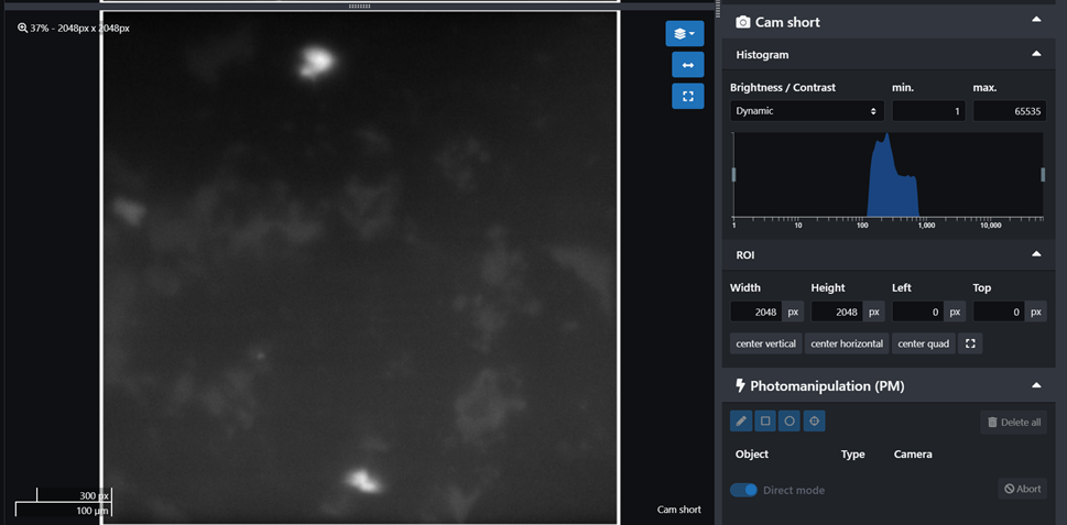
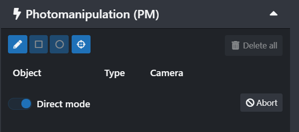
• Enable Photomanipulation. You can then adjust the ablation laser intensity and the other 3 parameters you need to set: The dwell time is the time the laser spot spends at each step. The number of repetitions can be increased if you want to repeat the ablation several times for a single z plane. The spacing controls the number of pixels covered by the ablation laser. Once you have defined an area or an object to be ablated, the total time it will take to perform the photomanipulation will appear in this window. 
• Set the appropriate filters for imaging. This will depend on your sample and selected illumination laser line, as in regular experiments. Make sure the ablation dichroic is selected! You should be able to image with the ablation dichroic. 

NOTE: Before running and experiment, check if the intensity of the object imaged with the ablation dichroic is within 10% of the intensity of the object imaged with an empty dichroic.

• When you enable Direct Mode you can choose to create a custom object with the little pencil icon.
• In order to create a rectangle of a circle shape you need to turn off the Direct Mode.
  
• Create the ablation pattern you want to perform and test it. You should see the laser spot ablate your sample according to the shape you chose. 

NOTE: We recommend that you experiment  with the photomanipulation on an area of your sample that does not present any interest before moving on to what you want to image in your experiment

Below is an example of ablation with a circular shape.

Set up an experiment with a PM event

Once you have decided on where and how to perform the photomanipulation, you need to set up the experiment.

A typical photomanipulation experiment should follow this format:

• Acquire a z-stack before any photomanipulation
• Perform the photomanipulation on selected z plane(s)
• Set the experiment for the duration you desire. For example, acquire a z-stack every 10 minutes for 24 hours.

Create a Channel for imaging

Always update the channel if any change is made! This channel should have all the imaging parameters you need: imaging laser, filters, camera parameters etc. 

Create a separate channel for the Photo-Manipulation event

Creating this extra channel is the safest way to run the PM module. This channel should have the cameras off and be turned on only during the PM event.

Create a z-stack

Create a PM object

Create Event 0

This is the event with the preliminary z-stack before photomanipulation.

Define the tasks:

Define a trigger:

Create Event 1

This is the event where the photomanipulation happens.

Define the tasks:

Make sure to select the channel created for the PM event for this event. Take note of the duration of the PM event so add a sufficient delay before starting the next event which is the imaging event of the experiment.

NOTE: As of April 2025, the software still runs all the events concurrently if the trigger is not properly defined! This is counter-intuitive. You should always calculate how long each event will take to run and then set the clock as such: Event_0 stars at time 0, Event_1 starts after the time it takes to run Event_0 and so on.

NOTE: Click on the settings icon next to the pm objects to define which z plane(s) should be photo-manipulated!

Define the trigger:

NOTE: Allowing the event to start after a few seconds is a good idea.

Create Event 2

This is the settings for the imaging experiment.

Define the tasks:

Set the trigger with a delayed start to make sure the PM event is fully completed:

Run the experiment

NOTE: Double check the triggers are set properly such that each event has time to run in order!!!

Always save your settings for future reference!

Look at the experiment with the image viewer in LuxBundle

• Select View last experiment or load your data in the Image Viewer.
• Select the imaging channels:

Go to the plane where you performed the ablation and you should be able to see it!

Current saving process with LuxBundle

As of November 2023, the software does not create a ims header or a big data viewer header for an experiment that contains a PM event. This is an error from LuxBundle and they are trying to fix it. Unfortunately, this bug also prevents the post-processing creation of ims headers. This means that you won't be able to look at your data in Imaris or Big Data Viewer by Fiji.

• Suggested work-around

Do not create an experiment that contains a PM event! Instead:

• • Acquire a single stack pre-PM event as experiment 1.
  • Perform the PM independently
  • Launch an experiment to image the stack  at several time points.

Always reach out to the Beckman center staff if you are in doubt about the process.

9. Bruker TruLive3D shut-down procedure

Once you are done with your experiment, please proceed with the following shut-down procedure:

• Turn off the microscope​

• Turn off the cameras​

• Turn off the chiller​

• Turn off the gas mixer controller​

• Close the CO2 valves

• Remove your sample from the chamber​

• Empty the sample chamber using the syringe. Be careful not to spill water. Dispose of the DI water that was in the chamber in the prep room and rinse the becher. Refill DI water squeezy bottle if needed.
  

• Dry the inside of the chamber using kimWipes and wipe everything using 70% ethanol. Wrap a kimWipe on a swab to access all areas in the chamber.

• Try not to touch the objective lenses while cleaning the sample chamber. NEVER use dry lens tissue, or worse - kimwipes, to clean the lenses as it may scratch them. If there is some unusual stain on the lenses it is best to contact Beckman Center staff immediately before attempting any sort of cleaning procedure. If you must clean them, use wet lens tissue or a microfiber swab with ethanol and go very gently.

• Close the lid once the chamber is dry.

• PLEASE wipe all areas you have used around the microscope, benches and desk with 70% ethanol. Do not leave your used gloves on the desk or benches.

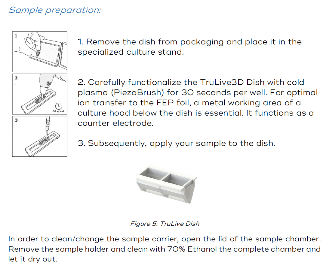
Bruker TruLive3D Sample preparation guidelines

This page contains some tips for sample preparation for the Bruker Trulive 3D. It is not exhaustive, it only gives a starting point for users on how to make their samples. Before planning an experiment, always check in with the Beckman center staff to ensure the sample preparation modalities will be compatible with the instrument.

1. Types of samples that can be imaged on the Bruker Trulive3D

The Bruker TruLive3D custom dishes allow for very specific imaging and their geometry is tailored to the instrument. While they are designed to give you optimal results with a variety of samples, they cannot accommodate everything.

Below is a picture of 3 dishes next to each other that fit into the sample chamber. Each cuvette has two sides separated by a plastic wall. 

\

These sample holders are made of a hard plastic structure and a thin foil where the specimen rests. This foil is specially engineered to match the index of refraction of water. 

The volume that can be imaged with the Bruker TruLive3D is defined by the working distance of the detection objective and the geometry of the dishes. Which is around 1 cubic millimeter. Samples bigger than 1mm in height and width will NOT fit into the dishes. You will have to cut them to dimensions.

The Bruker TruLive3D is specifically designed to image organoids and spheroids, small embryos, small zebra fishes, single cells. Samples that have an index of refraction equal or close to that of water (1.33) and are not optically dense will be easily imaged in the Bruker TruLive3D.

Samples that are too big or have an index of refraction higher than that of water will not be imaged well with the Bruker TruLive3D. For example, it is NOT designed to image brains or cleared tissues. The process used to clear tissues requires chemicals and some of them would actually attack the glue holding the detection objective in place, thus severely damaging the instrument. 

2. Immersion media

Once we agreed that your samples can be imaged with the Bruker TruLive3D, we need to define what is the immersion medium you need.

Ideally, your sample can be grown in a gel with an index of refraction equal to 1.33 or close to. Agarose and matrigel are good candidates. This is the best situation as it holds the specimen in place in the dish while allowing for growth if doing live imaging. It also helps preventing contamination as you can't spill the sample into the sample chamber.

You can also use some of your regular media in the dish BUT you will have to be extremely careful not to spill anything in the sample chamber as it is difficult to fully clean and sanitize.

3. How to prepare a sample in the Bruker TruLive3D dishes

Below are the recommendations given by Bruker about sample preparation:

Bruker TruLive3D emission filters and fluorophores spectrum

This page will help you select which filter combination you need for most commonly used fluorophores on the Bruker TruLive3D.

The Bruker TruLive3D light sheet microscope has two imaging cameras with two motorized filter wheels and two sets of filters. It is designed to split different emission wavelengths between the two cameras for simultaneous imaging with two different emission channels.

The "Long Camera" will record the fluorescence emitting at the longest wavelength and the "Short Camera" will record the fluorescence emitting at the shortest wavelength.

When you set up your experiment you want to make sure that you select the best filter option for each camera so that the fluorescence from one fluorophore does not mix up with the other.

The Bruker TruLive3D has the following emission filters options:

Filter wheel Short Camera: BP418-462    LP498    BP497-554    BP580-627   BP610-651

Filter wheel Long Camera:                         LP498    BP497-554    BP580-627    BP610-651    BP655-704

Below is a list of the most commonly used fluorophores and the filters you should use:

Fluorophores	Filter	Bruker Laser line
GFP	BP 497-554	488
DAPI	BP 418-462	405
TRITC	BP 580-627	561
mCherry	BP 580-627	561
AlexaFluor488	BP 497-554	488
AlexaFluor555	BP 580-627	561
AlexaFluor594	BP 580-627 or BP 610-651	561
AlexaFluor647	BP 655-704	640

To select the appropriate filters you need to know the emission peak wavelength of the fluorophores you are using.

For a better understanding on how to select the correct filter, you can look at the excitation/emission spectrums from fpbase.org   or aatbio.com for example. When you click on the link you can use the interactive spectrum viewer and see what the filters cover.

GFP : https://www.fpbase.org/protein/egfp/

mCherry : https://www.fpbase.org/protein/mcherry/ 

DAPI : https://www.aatbio.com/fluorescence-excitation-emission-spectrum-graph-viewer/dapi_4_6_diamidino_2_phenylindole

TRITC : https://www.aatbio.com/fluorescence-excitation-emission-spectrum-graph-viewer/tritc_tetramethylrhodamine_isothiocyanate

AlexaFluor488 : https://www.aatbio.com/fluorescence-excitation-emission-spectrum-graph-viewer/alexa_fluor_488

AlexaFluor555 : https://www.aatbio.com/fluorescence-excitation-emission-spectrum-graph-viewer/xfd555_alexa_fluor_555_equivalent

AlexaFluor594 : https://www.aatbio.com/fluorescence-excitation-emission-spectrum-graph-viewer/xfd594_alexa_fluor_594_equivalent

AlexaFluor647 : https://www.aatbio.com/fluorescence-excitation-emission-spectrum-graph-viewer/xfd647_alexa_fluor_647_equivalent

If your fluorophores are not on this page please let us know and we will update this page for you!

Bruker TruLive3D Data management pipeline

Bruker TruLive3D Data visualization in Fiji

The data generated by the Bruker TruLive3D contains a Fiji header named bdv.h5. 

Fiji is an open source software that can be very powerful to view, process and render your data. You should really explore its possibilities!

When you install Fiji (ImageJ) it comes with plugins and one of them is called BigDataViewer. This plugin has been specifically built to deal with Light-Sheet data. It will open the bdv.h5 file and allow you to visualize your stacks, plane by plane.

Fiji actually has an excellent documentation page on their website which I highly recommend reading and experimenting with!

Fiji BigDataViewer documentation

• When you drag the bdv.h5 file in Fiji this window will appear:

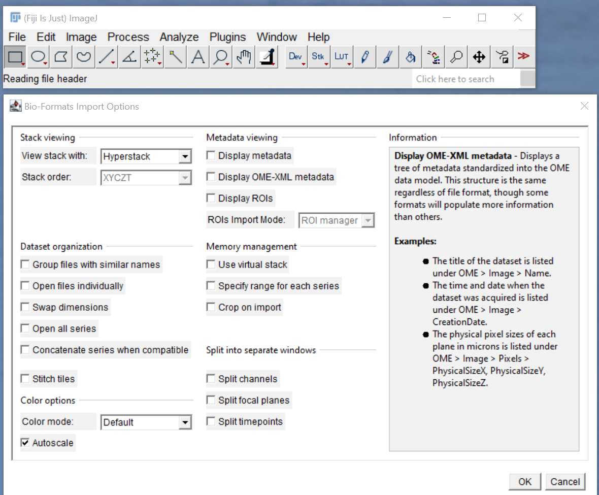
• Click ok
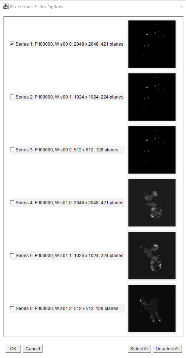
• This selection will appear for a single stack acquired with two channels:

  

• Series 1 and Series 4 are channel 1 and 2 in full resolution. You should select them both or one at a time to visualize the data in full resolution. Series 2, 3, 5 and 6 are lower resolution versions of the data in the two channels.

 

• Another useful plugin for Big Data in Fiji is BigDataProcessor. You can download it here.